I created QuantAscent because I wanted to find an edge in the stock market by picking my own stocks, and I believed that edge was in a company's financial statements rather than in chart patterns or day trading. Reading filings one company at a time doesn't scale, so I built software that scores every company on the same financial measurements and buys the best scores. The way it works is:
- You choose a universe, which is the list of stocks the software is allowed to pick from, by sector, company size, and minimum share price.
- It scores every company in that universe on a set of financial measurements called "metrics," such as profit margins, debt levels, and growth rates.
- It buys the highest-scoring companies.
- It holds them until your next rebalance, then re-scores the universe, sells the companies that no longer score high enough, trims or adds to the ones that do, and buys the new top scorers.
- You can pick the metrics yourself, or let statistical tests pick them for you and re-pick at each rebalance.
- Before you use a strategy with real money, you can test how it would have done in the past, and you can run thousands of variations at once to compare them.
A set of rules like that is what I mean by a strategy in this post.
Before I could release this to the public and ask people to pay for it in good conscience, there was one question I had to answer:
Does scoring stocks on their financial statements actually give you an edge?
If the answer is no, an index fund beats anything I could sell and I should go do something else. If the answer is yes, I want to know which feature is doing it.
So I used the software's sweep tool to build 31,000 adaptive strategies, the kind where the statistical tests pick the metrics, across 88 different universes from random combinations of settings, and I tested every one of them from 2016 to 2026. Each strategy was compared against two benchmarks: a random grouping of stocks from the same universe, and the ETF that matched its universe.
The answer
Yes, with caveats. Scoring stocks with statistical methods on their financial data definitively beat picking stocks at random. The median strategy made about 11% per year and beat 97% of the random portfolios drawn from the same stocks. Random picking made 2% per year. That said, the last time I checked there wasn't an ETF, or a sane person, that picks stocks at random as an investment strategy. So how did the strategies compare to their respective ETF benchmarks?
Against an ETF it was a mixed bag. On the broad universes that drew from every sector, the typical strategy landed about a point per year below the index. Sector by sector, it beat the ETF in energy, matched it in three sectors, and trailed it in the other seven. Table 1 shows the comparison between the strategies' compound annual growth rate (CAGR, i.e. the annual return) and their Sharpe ratio (a risk-adjusted return measure) against their benchmark.
| Sector | ETF | ETF CAGR | Strategy CAGR, mean ± 1 SD | ETF Sharpe | Strategy Sharpe, mean ± 1 SD |
|---|---|---|---|---|---|
| Energy | XLE | 10.9% | 13.0% ± 5.3 | 0.50 | 0.62 ± 0.18 |
| Industrials | XLI | 12.8% | 12.5% ± 4.2 | 0.74 | 0.72 ± 0.20 |
| Healthcare | XLV | 10.3% | 9.8% ± 3.9 | 1.04 | 0.73 ± 0.26 |
| Basic Materials | XLB | 9.3% | 8.7% ± 4.1 | 0.64 | 0.50 ± 0.17 |
| Financial Services | XLF | 12.3% | 10.1% ± 5.2 | 0.68 | 0.57 ± 0.21 |
| Consumer Defensive | XLP | 7.1% | 3.6% ± 3.1 | 0.75 | 0.34 ± 0.24 |
| Consumer Cyclical | XLY | 11.6% | 6.6% ± 4.2 | 0.68 | 0.41 ± 0.19 |
| Technology | XLK | 24.4% | 18.6% ± 5.8 | 1.17 | 0.94 ± 0.28 |
| Real Estate | XLRE | 5.5% | 1.7% ± 3.0 | 0.39 | 0.21 ± 0.13 |
| Communication Services | XLC | 12.7% | 6.8% ± 4.0 | 0.83 | 0.48 ± 0.23 |
| Utilities | XLU | 8.5% | 3.8% ± 2.7 | 0.64 | 0.37 ± 0.22 |
| All sectors, equal-weight picks | RSP | 11.3% | 10.2% ± 4.6 | 0.78 | 0.69 ± 0.28 |
| All sectors, cap-weighted picks | SPY | 15.0% | 14.0% ± 7.2 | 1.08 | 0.75 ± 0.31 |
Table 1. Each row is the strategies from one universe against that universe's ETF, over the ten years ending July 2026, before trading costs and taxes. The ± number is how much the strategies in that row varied with their settings.
Why should someone use this if it didn't beat the market in this test?
I had to do some serious soul searching after seeing the results. My hope was that the strategies would have all crushed their benchmarks. But the universe is never that kind. I considered giving up on this project completely and changing my own investment approach. But three things kept me going.
- People don't create strategies from random inputs. Testing randomly generated strategies and expecting them to beat the market is like throwing random ingredients in a pot and being surprised it doesn't win a cooking competition.
- ETFs don't let you choose which individual companies you invest in, or which ones you avoid.
- Investing in individual stocks lets you diversify across sectors, market caps, share prices, and filters in any combination you want. For example, see if you can find an ETF that holds technology, energy, healthcare, and basic materials companies, where every company has a market cap over $200 million, a share price over $10, and a positive free cash flow yield. You can't. I've checked. You'll have to take my word on this part, but I tested that exact idea in the software after I wrote the example. An adaptive strategy on those rules, holding 12 stocks, returned 310.5% from 2016 to 2026, which is about 15% per year with trading costs included. A random sample of settings can't account for a human making decisions like that.
Who should use this software
QuantAscent is for people who want to own individual companies and want rules, not a hunch or a tip, deciding which ones. You decide the universe, the software scores every company in it on its financial statements and keeps the portfolio current at each rebalance, and you can test any idea against the past before you put money into it. The software is a poor fit if what you want is the market's return with no work, because an index fund gives you that, and this study didn't show the software beating it.
If you'd rather just buy an index fund, you can stop reading here. But if you want to create your own strategies and have complete control over the stocks you invest in, keep reading to learn how I tested this idea, see the results in detail, and find out which settings produced the higher returns.
How I tested it
"Does it beat the market?" is the wrong first question. A portfolio of ten small companies and a cap-weighted index of the 500 largest companies aren't comparable, and the last decade was unusually good for the largest companies. So the first question was narrower: does the software pick better stocks than random chance would, from the same list?
That list is the universe. For every strategy, I drew 500 random portfolios from its universe, holding the same number of stocks the strategy held and redrawn every quarter, and counted how many of them the strategy beat. That count is its score. A strategy with no edge scores around 50. A strategy that beat 97% of the random portfolios scores 97.
I scored three things, because they don't move together: return, as CAGR; risk, as the worst peak-to-trough drawdown and separately as volatility; and return per unit of risk, as the Sharpe ratio. A method that makes the same return with half the drawdown has an edge. A method that makes 1% more with twice the drawdown doesn't.
The study ran on 88 universes so the answer wouldn't depend on any one choice: all eleven sectors together, each sector on its own, four sector groups, nine market-cap ranges from micro caps alone to all sizes together, and three filters, which were none, profitable companies only, or companies not in financial distress. One universe was chosen in advance as the main result: all sectors, all sizes, no filter. For each universe the sweep tool drew the settings at random, 500 times for the main universes and 200 times for the sector universes, and ran each draw as a complete strategy over the full ten years.
Beating random would show the software did something, but not which feature did it. So the main universes got four versions, run on the same stocks over the same quarters:
- Random picks used no financial data at all. This version scores 50 by definition, because it is the 500 random portfolios the others were measured against.
- Library only scored companies on the software's metric library, one metric per factor chosen at random, with no statistical test. This stands in for the Static Builder, where you choose the metrics yourself.
- Adaptive, any settings added the statistical test that chooses the metrics for you, with every setting sampled at random.
- Adaptive, shipped settings was the same thing on the default settings and the preset structures the app ships with, which it calls templates. This is the product as a new user first sees it.
A few terms come up in the results. The library's 77 metrics are grouped into 19 factors, such as margins, cash flow yields, valuation multiples, debt ratios, growth rates, and momentum, and each metric has a direction the textbook says it should work in: a higher return on capital is better, a higher debt-to-equity ratio is worse. A structure is the list of factors in a strategy and the weight on each. In an adaptive strategy you still choose the structure and how many companies to hold. The statistical test chooses the specific metric inside each factor and re-chooses it every quarter, using only data from before that date. If too few factors have a metric that qualifies, the strategy holds cash for the quarter.
The pass and fail thresholds were written down and committed to the repo before anything ran. EDGE meant the median strategy scored at least 60 with the uncertainty range clear of 50. HARM meant 40 or below with the range clear of 50. The range is a 95% range from a bootstrap, which means the ten years were re-drawn a thousand times, four consecutive quarters at a time in a random order with repeats allowed, every strategy was re-scored on each re-drawn decade, and the range is where the score landed 95% of the time. It's wide, because ten years is only 41 quarters. Everything in between was NOT DETECTED, because ten years of quarterly data can't tell a small edge from none. With 88 universes, about four would pass by luck alone if the method did nothing, so a broad claim needed more than eight.
The data covered about 6,700 US companies from 2009 to mid-2026, including roughly 2,000 that no longer exist, with the portfolio taking the loss when one was delisted mid-quarter. The ten years from August 2016 to July 2026 were scored. Every pick in this study was out of sample. At each rebalance, the statistical test used only data from before that date, and the following quarter's return was something it had never seen. The one thing that wasn't out of sample is the library itself. I chose which 77 metrics are in it, and which direction each one points, during the same years the study scores. The directions are the textbook ones, so there was little to fit, but it's still a bias in the software's favor that I can't remove. So every setting was drawn at random instead of chosen by me, and version 2 shows the library on its own, so you can see how much of the result rests on it.
Results
Everything below is an aggregate across strategies. No single run is "the strategy," no stock is named, and every number is before trading costs and taxes.
Table 2 is what the median strategy did in the main universe, every US stock over $5, for each of the four versions.
| Median run | 1. Random picks | 2. Library only | 3. Adaptive, any settings | 4. Adaptive, shipped settings |
|---|---|---|---|---|
| CAGR | 2.0% | 11.4% | 11.1% | 12.2% |
| Max drawdown | −47.4% | −31.1% | −25.4% | −25.5% |
| Volatility | 25.0% | 19.3% | 17.3% | 18.1% |
| Sharpe | 0.20 | 0.69 | 0.70 | 0.73 |
Table 2. The median strategy in the main universe for each version, August 2016 to July 2026. Random picking made 2% per year with a 47% worst fall. Every version that used the library made 11% to 12% per year with a worst fall of 25% to 31%.
Max drawdown is the worst fall from a previous high, and volatility is how much the portfolio's value moved from quarter to quarter.
Each strategy was also scored against random, and Figure 1 shows the median score for each version.
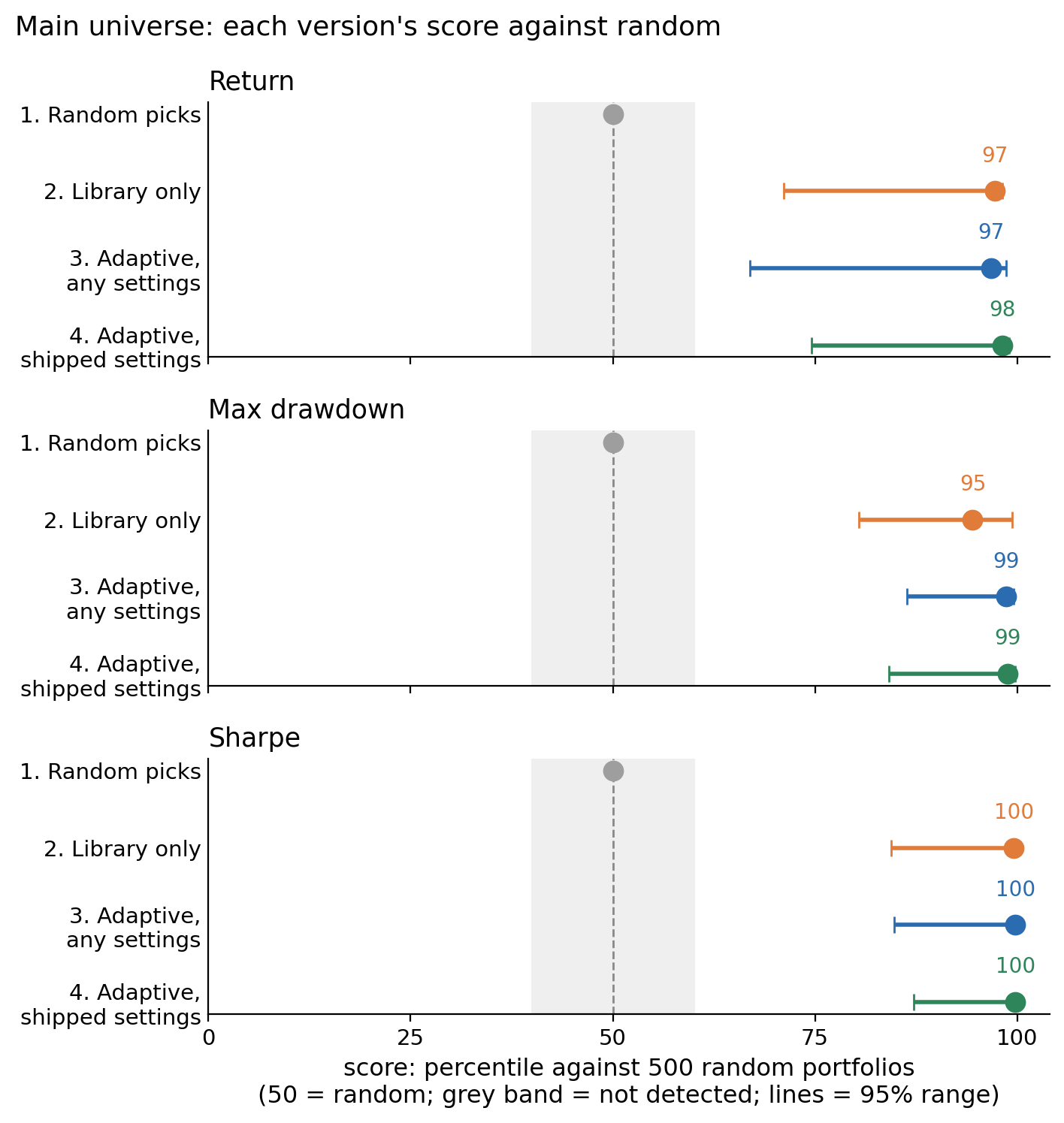
Figure 1. Each version's score against random in the main universe. The score is the share of 500 random portfolios the median strategy beat, so 50 means no better than random. The grey band is where the study called a result not detected, and the lines are the 95% range.
The median strategy scored 97 on return, 99 on drawdown, and 100 on Sharpe. That means it earned a higher return than 97% of the 500 random portfolios, had a shallower worst fall than 99% of them, and had a better return per unit of risk than nearly all of them. Before I ran this, I wrote down what I expected: the library beating a little under 60% of the random portfolios, only a bit better than a coin flip. I never would have guessed it would beat 97% of them. Why it did is the first finding below, and I think it's the most useful thing in this post.
The metric library did almost all of the work
The library is the heart of the software. It's the 77 financial-statement metrics QuantAscent computes for every US company every quarter, each with the direction the textbook says it should work in, grouped into 19 factors. Every strategy you build, static or adaptive, scores companies on it. Version 2 used nothing else: one metric per factor, chosen at random, no statistical test. It still scored 97 on return, 95 on drawdown, and 100 on Sharpe.
| Version | Runs | Return | Max drawdown | Sharpe |
|---|---|---|---|---|
| 1. Random picks | — | 50 | 50 | 50 |
| 2. Library only | 498 | 97 (71–98) | 95 (80–99) | 100 (84–100) |
| 3. Adaptive, any settings | 489 | 97 (67–99) | 99 (86–100) | 100 (85–100) |
| 4. Adaptive, shipped settings | 63 | 98 (75–99) | 99 (84–100) | 100 (87–100) |
Table 3. The scores from Figure 1 with their 95% ranges, written low to high, and the number of strategies behind each row. Every score in rows 2 to 4 met the EDGE threshold.
Random was this easy to beat because the universe was full of unprofitable companies. The main universe was about 3,700 companies per quarter, micro caps included. Owned in equal amounts, that whole universe compounded at 3.2% per year over the ten years, and the micro-cap portion alone lost 13.5% per year with an 82% drawdown. So a random ten-stock portfolio was mostly unprofitable companies, and scoring on the library avoided them.
In return terms, the median strategy in every version made 11% to 12% per year while the universe made 3%. Scoring companies on the library was worth about 8 points of annual return over random stock picking, and it didn't matter much which metric from a factor did the scoring. That's the biggest number in this study, and it comes from the part of the software every user runs, whether they build their strategies by hand or let the statistical test build them.
The statistical test removed the biggest losers
Switching the test on, with everything else held fixed, did nothing to the median return and a lot to the bad tail. Read left to right across versions 1 to 4, the return scores were 50 / 97 / 97 / 98, the drawdown scores 50 / 95 / 99 / 99, and the Sharpe scores 50 / 100 / 100 / 100. A score is a percentile and stops at 100, so the 5-point step I had set as the threshold for "the test adds something" couldn't be met from 97, and every step read NOT DETECTED. The fairer place to look is the median strategy's actual return and drawdown, which have no ceiling (Figure 2). The test took the median return from 11.4% to 11.1%, the worst fall from 31% to 25%, and volatility from 19% to 17%.
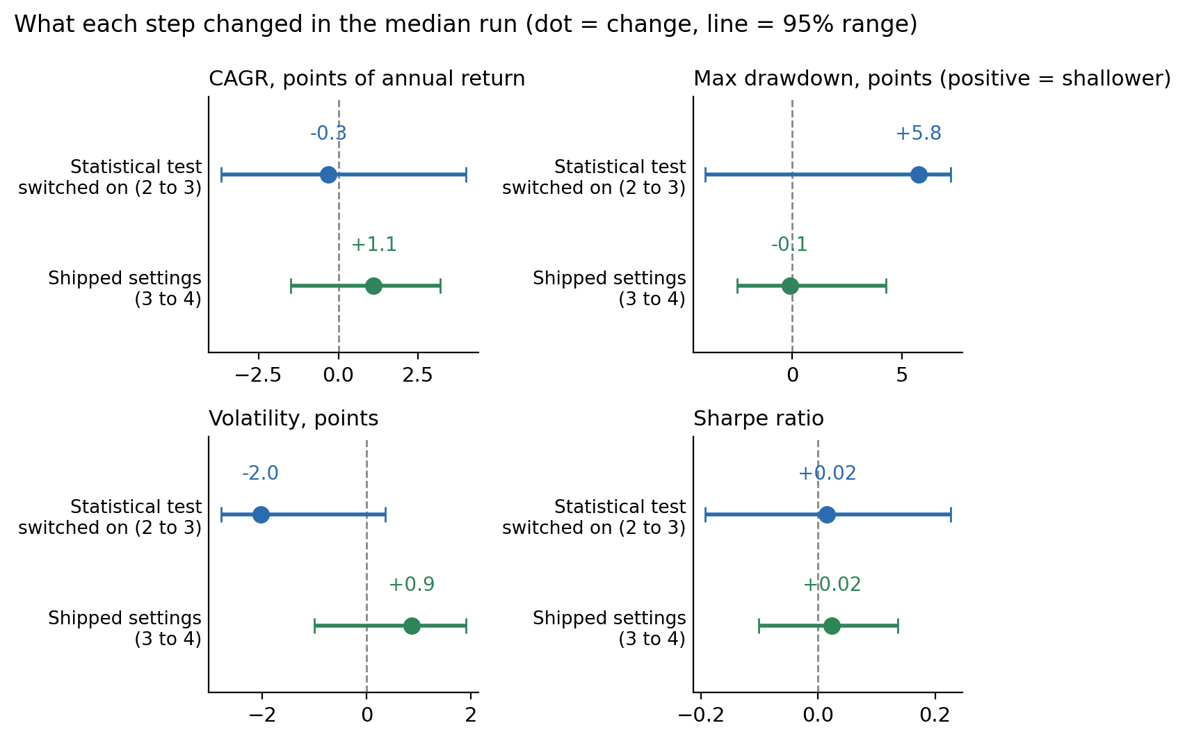
Figure 2. What each step changed in the median strategy, with its 95% range. The top row of each panel is the statistical test being switched on, and the bottom row is the shipped settings. The test took nothing off the return, made the worst fall about six points shallower, and cut volatility by two points.
I expected the return result from the design. The test chooses which metric represents a factor, never which factors, and two metrics from the same factor rank companies in much the same order.
Those numbers mix every kind of strategy the sweep built, including single-factor strategies and five-stock portfolios. A fairer test is to compare like with like: the same kind of strategy, blends of two or more factors holding 8 to 12 stocks, with the statistical test off and then on. Table 4 does that. The test cost about half a point of median return and cut the share of strategies with a 40%-or-worse drawdown from 17% to 6%. Its stricter settings pushed the same way: strict stability, the universe floor, and a higher signal floor each cut the share of deep drawdowns or low returns further, at a small cost in return. (Those settings are described in the method details near the end.)
| Same structures | Runs | Median CAGR | Median max drawdown | Runs with a drawdown of 40% or worse | Runs making under 5% per year | Runs beating the equal-weight S&P 500 |
|---|---|---|---|---|---|---|
| 2. Library only | 176 | 12.5% | −27% | 17% | 8% | 65% |
| 3. Adaptive, any settings | 176 | 11.9% | −24% | 6% | 7% | 54% |
| 4. Adaptive, shipped settings | 57 | 12.2% | −25% | 5% | 2% | 60% |
Table 4. Test off against test on at the same structures in the main universe. The last column is the share of strategies that beat RSP, the equal-weight S&P 500 ETF.
The other thing the test did was refuse to trade. Eleven strategies in version 3 never held a single stock in ten years, all of them on the pure "financial strength" template, because none of its metrics ever met the floor. Version 2 traded them and lost on them. Across every structure, the share of strategies that lost to random fell from 7.8% to 3.7%, the share making under 5% per year from 15.7% to 10.0%, and the share with a 40%-or-worse drawdown from 23.1% to 11.2%.
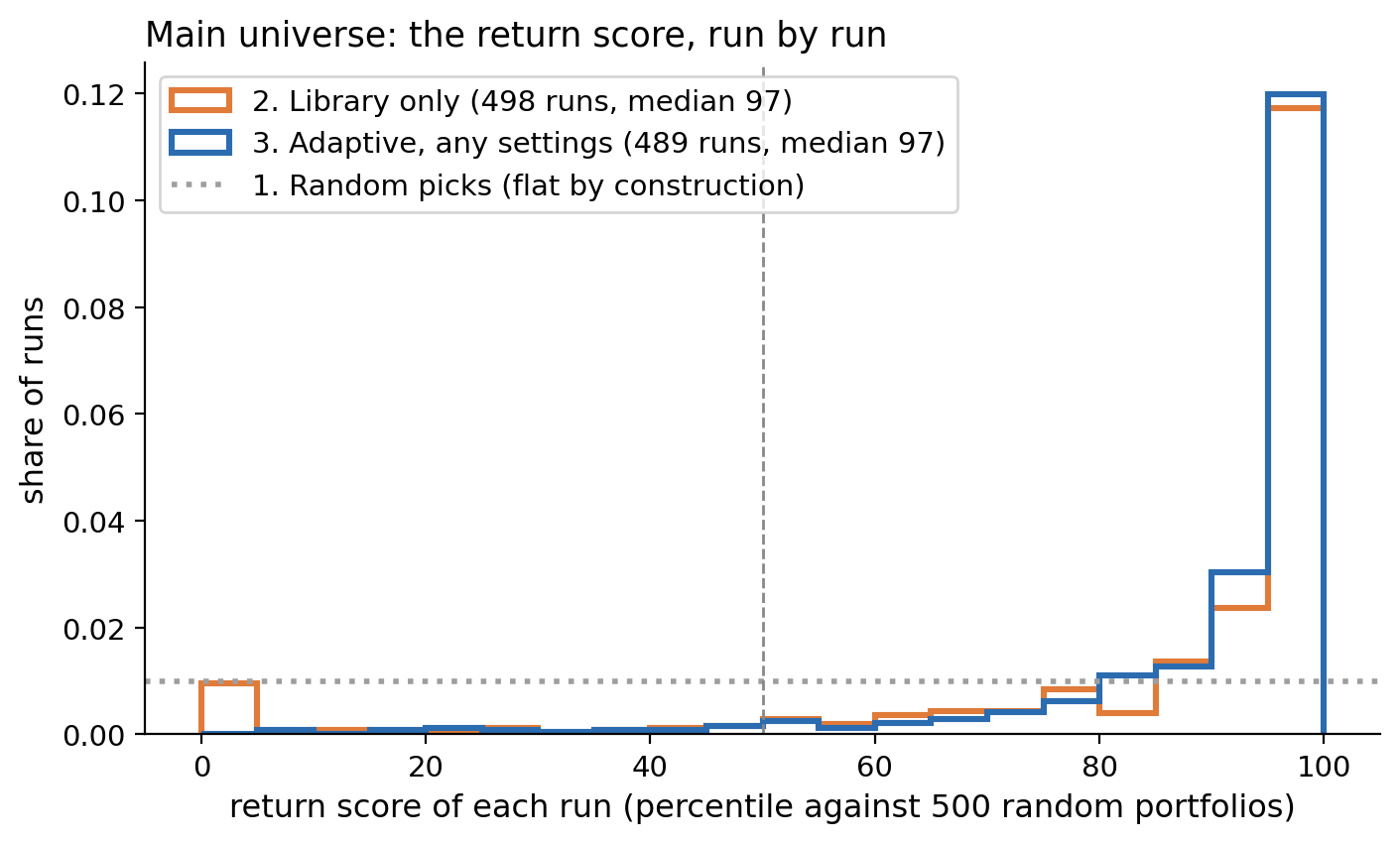
Figure 3. The return score of every strategy in the main universe for versions 2 and 3. A method with no edge would sit flat along the dotted line. Both versions pile up above 90, and the difference is at the far left, where version 2 has a small group of strategies that lost to almost every random portfolio and version 3 doesn't.
The statistical test didn't improve the best strategies. It removed the worst ones. 5% of version 2's strategies scored below the 12th percentile. 5% of version 3's scored below the 58th, and 5% of version 4's below the 81st.
Diversification was worth a point a year
Table 5 pools version 3 across the 28 main universes and shows the median return score for each setting.
| Choice | Setting | Return score | Median CAGR |
|---|---|---|---|
| Factors in the blend | 1 / 2 / 3 / 4 / 5 / 6 | 79 / 86 / 90 / 90 / 91 / 93 | 11.2% to 12.8% |
| Holdings | 5–7 / 8–11 / 12–15 | 85 / 89 / 92 | 11.7% to 12.4% |
| Training window | expanding / 12 / 16 / 20 / 24 quarters | 90 / 91 / 89 / 89 / 89 | about 12% throughout |
| How often the statistical test re-chooses | quarterly / every two years | 90 / 89 | |
| Stability | standard / strict | 90 / 88 | |
| Signal floor | 0.01 / 0.02 / 0.03 | 90 / 89 / 88 | |
| Universe floor | on / off | 90 / 89 |
Table 5. The median return score for each setting. More factors in the blend and more holdings each added about ten points. Every other setting moved the score by one or two.
Two rows move the score by about ten points, and the rest move it by one or two. The two are diversification: a blend of factors instead of one, and ten or more holdings instead of five. On the main universe, single-factor strategies made 10.4% per year and beat the equal-weight S&P 500 35% of the time, while blends made 11.2% and beat it 49% of the time. Strategies holding 5 to 7 companies made 10.1%, and strategies holding 8 to 15 made 11.3%. Both together, which is what the shipped defaults do, made 11.6% and beat it 53% of the time. Diversification had the second-largest effect in the study after the library itself, and it's your choice everywhere in the product.
The other rows are risk preference. The settings that tighten the statistical test cost a point of score and reduced deep drawdowns, and the training window and the re-choosing frequency changed almost nothing. The shipped defaults already use the settings that did best.
Backtests predicted risk, not return
Choose a date and treat it as the present. Every strategy's record up to that date is its backtest, and the two years after it are its future. Rank the strategies by backtest, rank them by future, and check whether the two rankings agree. I did this at four dates.
| Future window | Runs | Return: rank correlation | Drawdown: rank correlation |
|---|---|---|---|
| Aug 2018 to May 2020 | 485 | +0.34 | +0.32 |
| Aug 2020 to May 2022 | 478 | −0.08 | +0.22 |
| Jul 2022 to Apr 2024 | 485 | −0.09 | +0.22 |
| Jul 2024 to Jul 2026 | 489 | +0.14 | +0.27 |
Table 6. Whether a strategy's backtest predicted its next two years. A rank correlation of +1 would mean the backtest ranking held exactly, and 0 would mean it carried no information. Return reached the +0.20 threshold at one date of four. Drawdown reached it at all four.
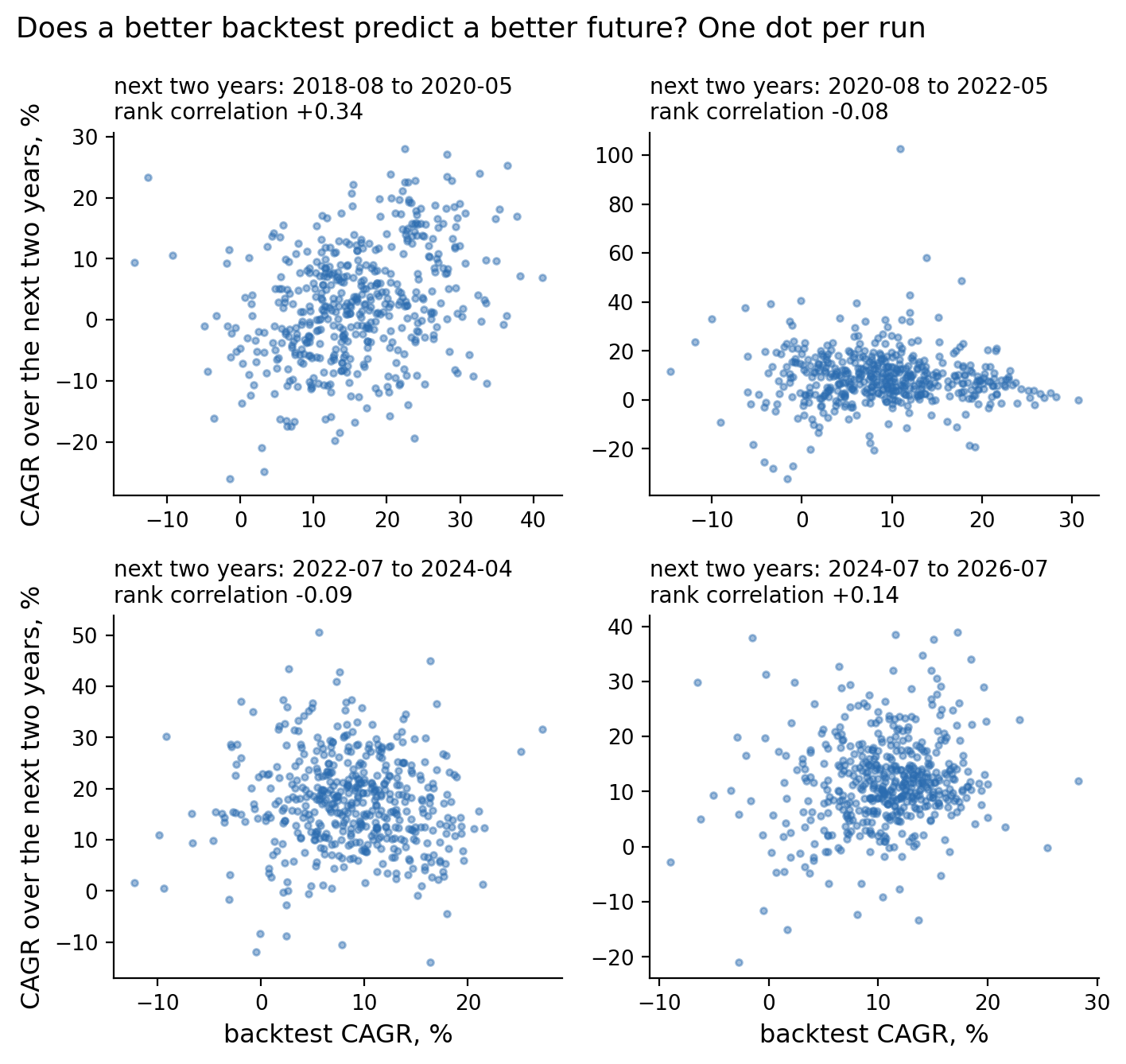
Figure 4. The same test with one dot per strategy, its backtest CAGR across the bottom and its CAGR over the next two years up the side. Only the first window has a visible slope. In the other three, a better backtest did not mean a better future.
Return DID NOT PERSIST and drawdown PERSISTED. If you had taken the top 10% of strategies by backtest return at each date and followed them for the next two years, they finished behind or level with the strategies they had outranked at three of the four dates, and ahead only in the first. This is why the sweep tool doesn't rank strategies by return. It's for seeing how a whole range of settings behaved, not for choosing a winner.
The app also shows every sweep run against a luck cutoff, which it calls the luck bar, and tells you two things: discard anything that doesn't clear it, and prefer the lower-risk runs. I applied both rules mechanically at each date and checked the next two years. Neither met the 5-point threshold at three of four dates, though the lower-drawdown runs did keep their lower drawdowns, just not strongly enough to count. The luck cutoff stays anyway, because its job is to stop you from treating a lucky run as a good one, not to find winners.
It matched the equal-weight S&P 500
The product holds every pick in equal amounts, so the fair index to compare it with is RSP, the equal-weight S&P 500 ETF, which made 11.3% per year over the ten years. The median strategy on the shipped settings made 12.2%, and the median sweep strategy made 11.0%. Depending on the version, 46% to 59% of the strategies finished ahead of RSP. By the rule I set before the run, which needed 60% or more ahead with the uncertainty range clear of 50%, that's a tie. In plain terms, the typical strategy did about what the equal-weight index did.
| Picks weighted | Version | Mean CAGR | Median CAGR | Matched index | Runs ahead |
|---|---|---|---|---|---|
| Equal | 2. Library only | 10.1% | 11.4% | RSP, 11.3% | 50% TIES |
| Equal | 3. Adaptive, any settings | 10.7% | 11.0% | RSP, 11.3% | 46% TIES |
| Equal | 4. Adaptive, shipped settings | 11.8% | 12.2% | RSP, 11.3% | 59% TIES |
| Cap | 2. Library only | 12.1% | 12.6% | SPY, 15.0% | 37% TIES |
| Cap | 3. Adaptive, any settings | 15.5% | 16.3% | SPY, 15.0% | 60% TIES |
| Cap | 4. Adaptive, shipped settings | 14.8% | 15.3% | SPY, 15.0% | 54% TIES |
Table 7. Each version against the index that weights the same way it does, on ten-year CAGR with cash earning zero in any quarter a strategy held no stocks. "Runs ahead" is the share of strategies that beat the index, and TIES means that share couldn't be told apart from 50%.
The comparison everyone asks about, equal-weight picks against the regular cap-weighted S&P 500, isn't a fair one, because SPY made 15.0% per year by holding the giant companies in giant size. Only 13% to 25% of the strategies beat it. So as a side calculation I re-weighted the same picks by market cap and compared them with SPY. That brought the median strategy to 16.3% per year, and 60% of them finished ahead of SPY (Figure 5). For scale, S&P's own scorecard finds that about 14% of actively managed large-cap funds beat the S&P 500 over the ten years to 2025, after fees. Strategies with randomly chosen settings matched that rate before costs at equal weight, and the cap-weighted version of the same picks beat it four times over, with the caveat below about what one decade can prove.
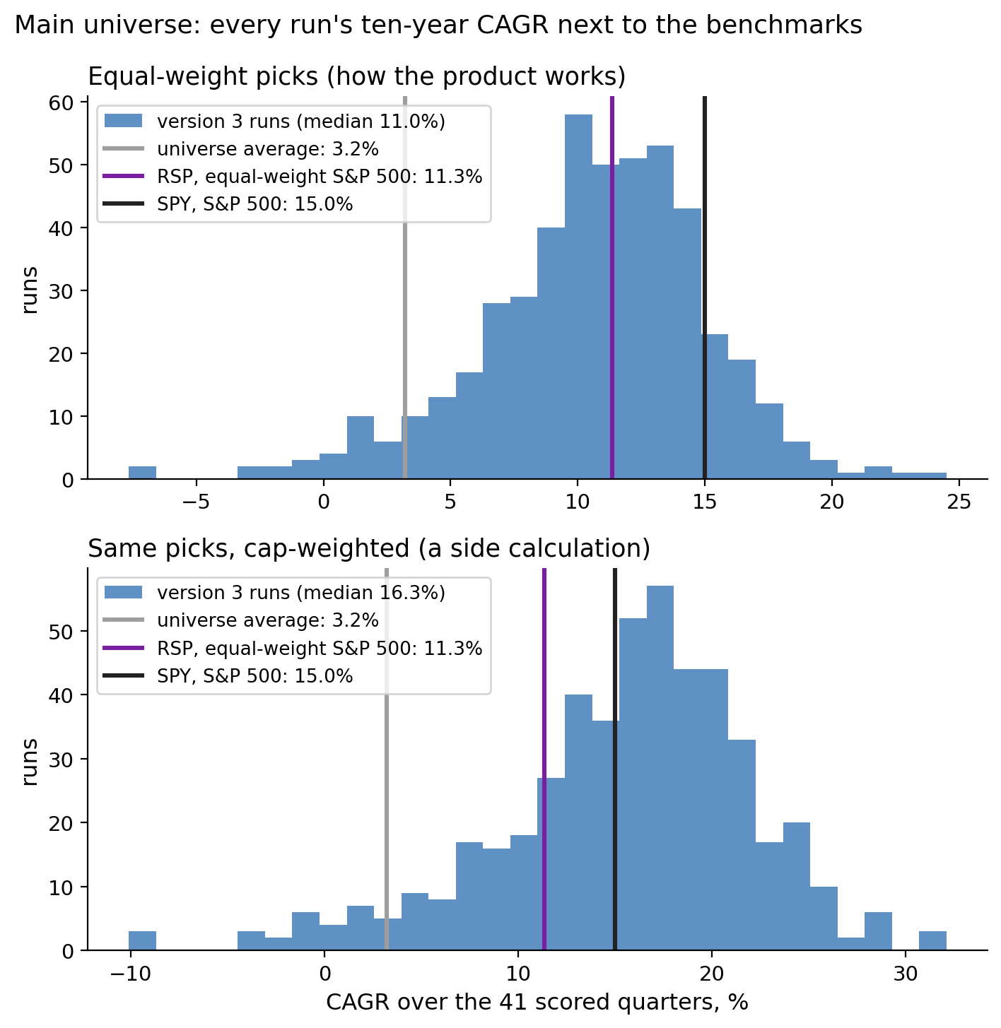
Figure 5. Every version 3 strategy's ten-year CAGR in the main universe, with the benchmarks as vertical lines. In the top panel the picks are held in equal amounts, the way the product works, and the strategies center on RSP. In the bottom panel the same picks are weighted by market cap, and most strategies sit to the right of SPY.
So why does Table 7 still say TIES for that row? Because SPY's 15% came from a few enormous quarters, and the test asks whether the result would hold in a different ten years. The bootstrap, the same one behind every range in this post, re-drew the decade a thousand times. In the draws that included those big quarters twice, 23% of the strategies beat SPY. In the draws that missed them, 80% did. That range includes 50%, so the rule calls it a tie. The 60% is real for the decade that happened. Whether it was the method or the decade's mix of quarters, ten years can't say.
Cap weighting was also where the statistical test mattered most. Switching it on moved the cap-weighted median from 12.6% to 16.3% per year and the share beating SPY from 37% to 60%. The ranges on those steps reached just below zero, and the cap-weighted comparison was registered as secondary before the run, so it can't carry a verdict on its own. It's the first thing I'd test next.
Two caveats on this section. Dead-company coverage in the data is a handful of companies per year before 2016, which is why the scoring starts there, and only partial from 2016 to 2020. Missing dead companies raise the software's returns but not the index's, so this comparison leans in the software's favor. Trading isn't free, and none of the numbers in this post include its cost. The typical strategy sold and replaced about seven of its ten stocks every quarter, which comes to roughly 60 trades a year. Using the app's default assumptions of $1 per trade plus a small price concession on each one, that costs about 1% of a $10,000 account per year, and about two thirds of 1% on a $100,000 account. So knock up to a point off every return in this post, depending on your account size.
For completeness, every version also beat owning every stock in the universe in equal amounts, which made 3.2% per year. 89% to 97% of the strategies finished ahead of that, and all three versions read BEATS.
The edge held in every two-year window
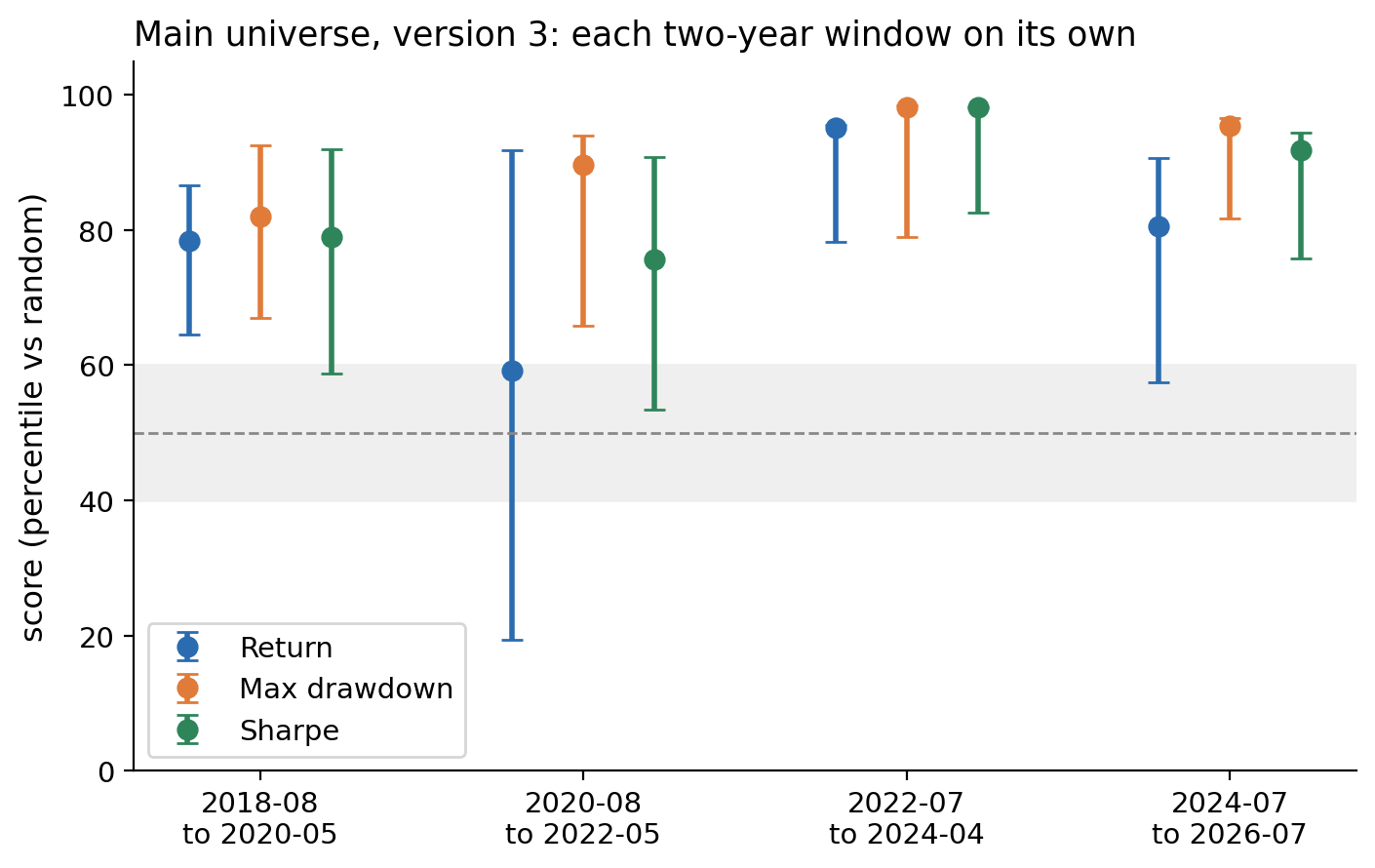
Figure 6. Version 3's return, drawdown, and Sharpe scores in the main universe for each two-year window on its own, with 95% ranges. The grey band is the not-detected zone. The only dot inside it is return in the window beginning August 2020.
| Window | Runs | Return | Max drawdown | Sharpe |
|---|---|---|---|---|
| Aug 2018 to May 2020 | 485 | 78 (65–87) | 82 (67–93) | 79 (59–92) |
| Aug 2020 to May 2022 | 478 | 59 (19–92) n.d. | 90 (66–94) | 76 (53–91) |
| Jul 2022 to Apr 2024 | 485 | 95 (78–96) | 98 (79–98) | 98 (83–98) |
| Jul 2024 to Jul 2026 | 489 | 81 (57–91) | 95 (82–97) | 92 (76–94) |
Table 8. The scores in Figure 6 as numbers. Eleven of the twelve cells met the EDGE threshold. The one that didn't is marked n.d., for not detected.
Eleven of the twelve cells in Table 8 met the EDGE threshold. The one that didn't was return in the window that began in August 2020, during the rally in unprofitable small companies, when random portfolios of micro caps did well for a while. Risk held in every window. That was the pattern of the whole study in one window.
Where it worked and where it didn't: 88 universes
This is version 3 on all 88 universes over the full ten years. Chance alone would have produced EDGE on about 4 of them, with an upper bound of 8.
| Test | EDGE | NOT DETECTED | HARM |
|---|---|---|---|
| Return | 29 | 57 | 2 |
| Max drawdown | 43 | 45 | 0 |
| Volatility | 52 | 36 | 0 |
| Sharpe | 43 | 43 | 2 |
Table 9. Verdicts across all 88 universes. EDGE meant the median strategy scored at least 60 with the range clear of 50, HARM meant 40 or below, and everything else was NOT DETECTED. Return reached 29 universes, and the other three measures reached 43 to 52.
Return met the threshold, and risk passed it by a wider margin. The two HARM universes on return were both utilities with the profitability filter on.
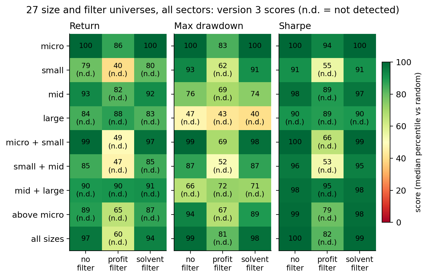
Figure 7. Version 3's median score in each of the 27 size and filter universes drawn from all sectors. Rows are company-size ranges and columns are the universe filter. Darker green is a higher score, and n.d. marks a universe that didn't meet the EDGE threshold.
Three results in Figure 7 were worth the whole study to me.
The profitability filter removed most of the return edge. Filtering the universe to profitable companies first dropped the return score to 40 for small caps and 60 for all caps, neither distinguishable from random. Once the unprofitable companies were out, the random portfolios were no longer full of them, and the software stopped beating them on return. Risk still improved in most of those universes. This is the cleanest statement of what the library does: it avoids unprofitable companies. Once those were filtered out, neither the library nor the statistical test picked better among the survivors on return.
Large caps showed no risk edge. The drawdown scores were 40 to 47 across the three filters. Random portfolios of large companies were already diversified and solvent, and the software's picks had drawdowns about as deep as theirs.
Micro and small caps showed the biggest edge, and they're the ones that can't absorb much money. Micro caps scored 100 on everything, with or without a filter, because the alternative was minus 13.5% per year.
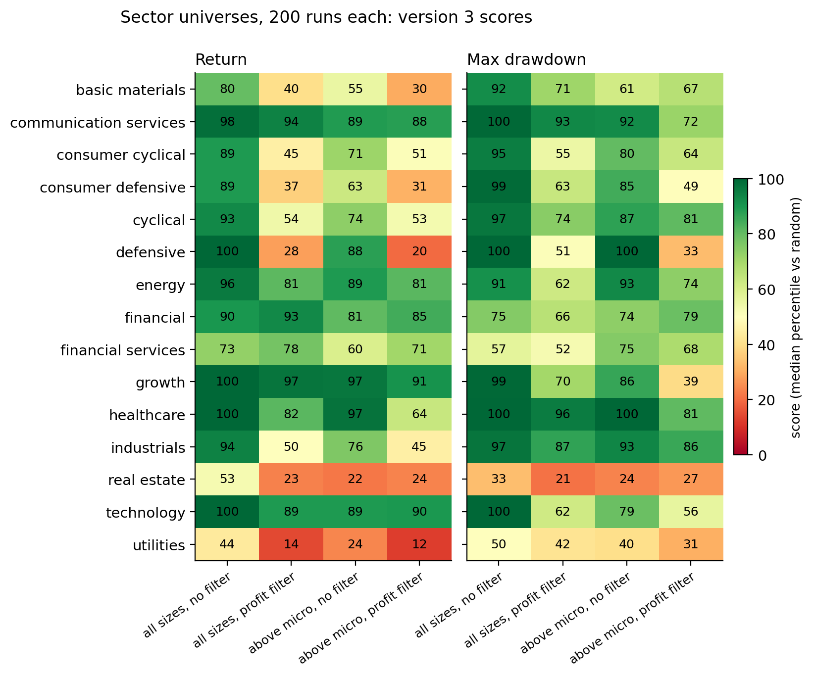
Figure 8. Version 3's median return and drawdown scores for the 60 sector universes, about 200 strategies each. The growth row is technology plus communication services. Utilities and real estate were the only sectors below 55 on return in every combination.
The sector universes split the same way. Technology, the technology-plus-communications group, healthcare, communication services, and energy scored 89 to 100 on return. Utilities and real estate scored 12 to 24 in three of their four combinations. Against the sector ETFs, no universe reached the 60% threshold. Technology picks beat XLK 11% of the time, because XLK compounded at 24% per year, and energy picks beat XLE 68% of the time in one of its four combinations but not consistently across all four. "Beats random stock picking inside the sector" and "beats the sector ETF" are different claims, and only the first one held.
One more result, reported because the rule said every universe gets reported. In one of the nine no-filter universes, small caps, switching the statistical test on cost 12 points of return score with a range clear of zero. One of nine at the 5% level is what chance predicts.
What it means if you use the software
The library is the core product. Scoring companies on its metrics in their textbook directions, with no test choosing among them, took the median strategy from 2% per year to 11.4% and to the 97th percentile against random in the main universe. It scored above random in most of the 88 universes, cleared the strict threshold on return in 29 of them against the 8 that chance could produce, and held in every two-year window. That scoring runs inside every strategy you build, in the Static Builder as much as in adaptive strategies. It's the core of QuantAscent: the metric set, the directions, the financial-statement data for every US company, and the re-scoring at every rebalance, in one place.
Adaptive strategies did their work on drawdowns, not on return. At the same structures, the statistical test cut the share of strategies with a 40%-or-worse drawdown from 17% to 6%, cost about half a point of median return, and refused to run factors with no signal. It didn't find return, and in this design it can't, because it chooses within factors rather than between them.
Strategies that blended factors and held ten or more companies did about a point a year better. The gap over a single factor and five holdings was about a point of annual return and ten points of score. The product lets you choose it everywhere, and the defaults already do.
The other settings moved the result a point or two either way. The ones that tighten the test trade return for fewer deep drawdowns.
The sweep tool compares settings. It doesn't find winners. Backtest return didn't predict future return at any useful strength. Backtest risk did. The app keeps listing every run without ranking them by return.
Method details
How the 88 universes were built. A universe came from three choices: which sectors, which company sizes, and whether to apply a filter. The size bands were micro caps under $300 million, small caps from $300 million to $2 billion, mid caps from $2 billion to $10 billion, and large caps at $10 billion and up with no upper limit, so the mega caps were in the large band. The main set crossed every size range with every filter on all sectors, which made 27 universes, plus one reference universe with the textbook distress threshold. The sector set took each sector and sector group at two sizes, with and without the profitability filter, which made 60 universes. The minimum share price was $5 throughout.
How the settings were sampled. For each universe, the settings were drawn at random from every factor, blends of one to six factors, 5 to 15 holdings, every training window and re-choosing frequency the app offers, both stability options, signal floors of 0.01, 0.02, and 0.03, and the universe floor on or off. The app allows more in places, and the study's ranges were chosen to cover what a typical user would set. Samples that came out identical were merged, which is why some universes show 494 to 500 runs rather than exactly 500. The study covered only the library's own directions. Reversing a direction is allowed in the software, and the study did not grade it.
What an adaptive strategy's settings are. The training window is all available history or the trailing 12, 16, 20, or 24 quarters. The test re-chooses its metrics every quarter or about every two years. The signal floor is the minimum average strength a metric needs to qualify. The stability setting decides whether each half of the training window must meet the floor on its own. The universe floor, when on, lets the test remove the weaker half of the universe before scoring, using the one metric whose top and bottom halves had the biggest gap in returns over the training window. All of them ship with defaults, and the exact rules are in the math section.
How the random portfolios were drawn. Each random portfolio held the same number of companies the strategy actually held that quarter, and was redrawn every quarter from the strategy's own universe. The 2.0% in Table 2 is the median over the 244,500 random portfolios the strategies were graded against. It's below the 3.2% universe average because a ten-stock random portfolio has the same average return as the universe but much more variation, and the median outcome of a volatile portfolio is below its mean.
How the backtest-predicts-future test was set up. The four dates had futures ending May 2020, May 2022, April 2024, and July 2026. The threshold was a rank correlation of +0.20 or better at three of the four dates. The app's two pieces of advice, discard anything below the luck cutoff and prefer the lower-risk runs, were applied mechanically at the same four dates, with a 5-point lead at three of four dates as the threshold.
The data. About 6,700 US companies, 3,000 to 5,000 in any given quarter, quarterly from 2009 to mid-2026, from a commercial fundamentals vendor. The scored quarters were August 2016 through July 2026, 41 in all, and 2009 to 2016 was training history only. The roughly 2,000 dead companies were found through exchange delisting filings. Coverage of those delistings was dense from 2021 on, partial from 2016 to 2018, thin in 2019 and 2020, and essentially absent before 2016, which is why nothing before 2016 was scored. That gap, which I call the survivorship gap elsewhere in this post, raised the returns of the software, the random portfolios, and the universe average equally, so the comparison against random was clean. It raised the software's returns against the market, and I say so where it matters. Companies trading under $1 today were missing entirely, history included, and both sides shared that gap.
Costs. Every number was before trading costs and taxes. The app's backtester applies a cost model, but the records of adaptive strategies come from the walk-forward engine the study ran, which the app's own record cards label as gross. Turnover was measured so the cost could be estimated, and the estimate is in the market section above.
The math, for anyone checking
Nothing above depends on this section. It is here so that "edge," "risk," and "beats random" are exact, and so that the work can be checked. Every equation is followed by a list of what each symbol means.
Every portfolio produced one return per quarter, \(r_t\): the equal-weight average of its holdings' 90-day total returns, dividends included, with each company's return capped at plus or minus 100%. Compounding those returns gave a wealth path \(W_t\).
$$ r_t = \frac{1}{N_t}\sum_{i \in P_t} \min\!\big(1,\;\max(-1,\; R_{i,t})\big), \qquad W_0 = 1, \quad W_t = W_{t-1}\,(1 + r_t) $$
where:
- \(t\) is the quarter, counting from 1 to \(T\), the number of quarters in the span
- \(i\) is a company
- \(P_t\) is the set of companies held in quarter \(t\), and \(N_t\) is how many
- \(R_{i,t}\) is company \(i\)'s dividend-adjusted return over the 90 days after the rebalance date, and the min and max cap it at plus or minus 100%
- \(W_t\) is the wealth path: what one dollar invested at the start had grown to after quarter \(t\)
Three measures were defined on that path over \(T\) quarters:
- Return, as compound annual growth rate: $$ \mathrm{CAGR} = \left(\frac{W_T}{W_0}\right)^{4/T} - 1 $$ Excess return, when a benchmark was involved, was the portfolio's CAGR minus the benchmark's over the same \(T\) quarters.
- Max drawdown, the worst fall from the highest point the wealth path had reached so far. First find that running high, then take the worst drop below it: $$ \mathrm{Peak}_t = \max(W_0, W_1, \dots, W_t), \qquad \mathrm{MaxDD} = \min_{1 \le t \le T} \left( \frac{W_t}{\mathrm{Peak}_t} - 1 \right) $$
- Volatility: the sample standard deviation of the quarterly returns (how far each quarter's return \(r_t\) is from the average return \(\bar{r}\), squared, averaged with the usual \(T - 1\) correction, square-rooted), then annualized by the square-root-of-time rule, which for 4 quarters per year is \(\sqrt{4}\): $$ \sigma_{q} = \sqrt{\frac{1}{T - 1} \sum_{t=1}^{T} \left( r_t - \bar{r} \right)^2 }, \qquad \sigma = \sqrt{4}\;\sigma_{q} $$ Returns are simple returns, not log returns, because they are what the wealth path compounds.
- Sharpe ratio: the average quarterly return divided by the quarterly volatility, annualized by the same \(\sqrt{4}\), with the risk-free rate set to 0 (the app's convention): $$ \mathrm{Sharpe} = \sqrt{4}\;\frac{\bar{r}}{\sigma_{q}} $$
Each measure was scored as a percentile against the random portfolios. With \(m\) the run's value of a measure and \(m_k\) the value for the \(k\)-th of 500 random portfolios over the same quarters:
$$ p = \frac{100}{500} \sum_{k=1}^{500} \mathbf{1}\big[\, m \text{ beats } m_k \,\big] $$
where:
- \(k\) counts the random portfolios, 1 to 500
- \(\mathbf{1}[\,\cdot\,]\) is the indicator function: 1 when the statement inside is true, 0 when it is false, so the sum is a count of random portfolios beaten
- "beats" means higher for CAGR and Sharpe, shallower for max drawdown, and lower for volatility, so higher is always better, and 50 always means "indistinguishable from random"
Every interval came from a block bootstrap. Runs within a universe share quarters, so they are nowhere near independent. Every interval was a 4-quarter circular block bootstrap over the span's quarters, with 1,000 resamples: resample blocks of four consecutive quarters, recompute every run's and every random portfolio's measure on the resampled path, then recompute the scores and the cross-run median. The backtest-predicts-future test was the Spearman rank correlation across runs between CAGR over the backtest period and CAGR over the two years after, and separately for max drawdown. The comparison between versions was the difference in cross-run median scores, with a 5-point minimum difference and a bootstrap interval on the difference, computed on identical resampled paths for both versions.
An adaptive strategy repeated the following at every rebalance date. Take a rebalance date. The training window \(\mathcal{T}\) is the set of past quarters the training-window setting allows (all of them, or the trailing 12 to 24). Split it into an early half \(\mathcal{T}_1\) and a late half \(\mathcal{T}_2\). Everything below was computed from those quarters only.
Step 1 measured each metric. The question for metric \(j\) on a past date \(t\) was: if you had sorted every company in the universe by this metric on that date, how closely would that order have matched the order of their returns over the next 90 days? That is a Spearman rank correlation across the companies on that date, written \(\mathrm{IC}_{j,t}\) (the information coefficient). A metric's signal in each half of the window was the average of its per-date correlations:
$$ \mathrm{IC}_{j,t} = \rho_{\mathrm{S}}\!\left( x_{j,i,t},\; R_{i,t} \right)_{i \in U_t}, \qquad \overline{\mathrm{IC}}_{j,h} = \frac{1}{|\mathcal{T}_h|} \sum_{t \in \mathcal{T}_h} \mathrm{IC}_{j,t}, \quad h \in \{1, 2\} $$
where:
- \(j\) is the metric and \(t\) is the date
- \(U_t\) is the universe on date \(t\), the set of companies the process could choose from, and \(i \in U_t\) says the correlation runs across those companies
- \(x_{j,i,t}\) is company \(i\)'s value of metric \(j\) on date \(t\), and \(R_{i,t}\) is its return over the next 90 days
- \(\rho_{\mathrm{S}}\) is the Spearman rank correlation: rank the companies by the metric, rank them by the return, and measure how well the two rankings agree, from \(-1\) to \(+1\)
- \(h\) is the half of the training window, 1 for early or 2 for late; \(\mathcal{T}_h\) is the set of dates in that half and \(|\mathcal{T}_h|\) is how many dates it holds
- \(\overline{\mathrm{IC}}_{j,h}\) is the metric's average IC over that half
\(\rho_{\mathrm{S}}\) is itself a calculation, and everything in it happens on one date. Nothing looks across time. The averaging over dates happens one level up, in \(\overline{\mathrm{IC}}_{j,h}\). This is what statisticians call cross-sectional: a single snapshot of all the companies side by side. On that date, give every company in the universe two ranks, \(a_i\) for where it ranks on the metric and \(b_i\) for where it ranks on the return, with 1 the best. Spearman's correlation is the ordinary correlation of those two rank lists:
$$ \rho_{\mathrm{S}} = \frac{\sum_{i} (a_i - \bar{a})(b_i - \bar{b})}{\sqrt{\sum_{i} (a_i - \bar{a})^2 \;\cdot\; \sum_{i} (b_i - \bar{b})^2}} $$
where:
- \(i\) is a company, and the sums run over the \(n\) companies in the universe on that one date
- \(a_i\) is company \(i\)'s rank by the metric among those \(n\) companies, and \(b_i\) its rank by the return among the same companies
- \(\bar{a}\) is the average of the metric ranks across the companies on that date, and \(\bar{b}\) the average of the return ranks. With \(n\) companies ranked 1 to \(n\), both averages equal \((n+1)/2\), the middle rank. So \(a_i - \bar{a}\) is how far above or below the middle company \(i\) is on the metric that day, and \(b_i - \bar{b}\) the same for its return; they are not comparisons with the company's own history
A company that is above the middle on both lists, or below the middle on both, adds a positive term to the numerator. A company high on the metric but low on the return adds a negative one. The denominator only scales the result to run from \(-1\) to \(+1\).
You may recognize the shortcut version from a textbook, \(\rho_{\mathrm{S}} = 1 - 6 \sum_i d_i^2 / \big(n (n^2 - 1)\big)\), with \(d_i = a_i - b_i\) and \(n\) the number of companies. It gives the same number as the formula above only when no two companies tie, and ties happen on every date in this data, so the software always uses the general form above, with tied companies given the average of the ranks they span. The shortcut is here for recognition only. Identical rankings give \(+1\), reversed rankings give \(-1\), and no relationship gives about 0. On real data a single metric on a single date was usually between \(-0.1\) and \(+0.1\). The signal is faint, which is why the floor in the next step is as low as 0.02. The question is whether it is faint in the same direction, consistently.
Averaging the per-date correlations, instead of running one big correlation over all dates at once, matters. It stops a bull quarter from outweighing a bear quarter, and it stops a date with 4,000 companies from outweighing one with 400.
Step 2 decided which metrics qualified. Every metric comes with a direction the textbook says it should work in, \(d_j = +1\) (higher is better, like return on capital) or \(d_j = -1\) (lower is better, like debt to equity). That direction is fixed and was never fit to the data. A metric qualified when three things were true: its average IC had the textbook sign in the early half, it had the textbook sign in the late half, and its average strength was at or above a floor \(\mathrm{IC}_{\min}\), a setting between 0.01 and 0.03:
$$ d_j\,\overline{\mathrm{IC}}_{j,1} > 0, \qquad d_j\,\overline{\mathrm{IC}}_{j,2} > 0, \qquad \tfrac{1}{2}\left| \overline{\mathrm{IC}}_{j,1} + \overline{\mathrm{IC}}_{j,2} \right| \ge \mathrm{IC}_{\min} $$
where the vertical bars are absolute value, so the third condition reads "the average of the two halves, ignoring sign, is at least the floor." It also needed at least 500 valid company-dates in the window. The strict setting required each half on its own to meet the floor, not just the average.
Step 3 filled the slots. A structure is a list of slots. Each slot names a factor (margins, momentum, leverage, and so on) and has a weight \(w_c\). Each slot took the qualifying metric from its factor with the strongest average signal, \(\tfrac{1}{2}\left|\overline{\mathrm{IC}}_{j,1} + \overline{\mathrm{IC}}_{j,2}\right|\). If fewer than two slots could be filled, the process held cash that quarter rather than trade on a rule it could not build. Version 2 replaced only this step: each slot took a uniformly random metric from its factor, scored in the library's direction, with no test and no floor.
Step 4 scored the companies and picked the portfolio. On the current date, each chosen metric was turned into a 0 to 100 percentile rank across the universe, with 100 being the best in that metric's direction. The composite score was the weighted average of those ranks:
$$ S_i = \sum_{c} w_c \; \mathrm{pct}_{c,i} $$
where:
- \(c\) is a slot in the structure
- \(w_c\) is the slot's weight, after the weights have been scaled so they add up to 1
- \(\mathrm{pct}_{c,i}\) is company \(i\)'s percentile rank on the metric that fills slot \(c\)
- \(S_i\) is company \(i\)'s composite score, so a company at the 90th percentile on every slot scores 90
Buy the top \(N\) by \(S_i\), equal weight, hold one quarter.
The universe floor was an optional step before scoring. With this setting on, the universe was cut in half on one metric before scoring. The metric was chosen like this: for each candidate metric and each training date, split the universe at that date's median value of the metric, and take the average return of the companies above the median minus the average return of those below it. Average that gap over the training dates (requiring at least 8 dates, each with at least 40 companies and 15 on each side):
$$ L_j = \frac{1}{|\mathcal{T}|} \sum_{t \in \mathcal{T}} \left( \overline{R}_{\,x_{j} > \mathrm{med}_t(x_j)} - \overline{R}_{\,x_{j} \le \mathrm{med}_t(x_j)} \right) $$
where:
- \(\mathcal{T}\) is the training window and \(|\mathcal{T}|\) is the number of dates in it
- \(\mathrm{med}_t(x_j)\) is the median value of metric \(j\) across the universe on date \(t\)
- \(\overline{R}_{\,x_j > \mathrm{med}_t(x_j)}\) is the average next-quarter return of the companies above that median, and \(\overline{R}_{\,x_j \le \mathrm{med}_t(x_j)}\) the average for those at or below it
- \(L_j\) is the metric's average gap between the two halves, the lift
The floor metric was the one with the biggest gap \(|L_j|\) whose sign agreed with its textbook direction. At deployment, the universe kept the companies on the better side of that quarter's median of that metric. It never removed more than half.
All of this was redone at every rebalance date using only the quarters before it. That is what made every scored quarter out of sample: the rule in force on a date was built without seeing that date's returns.
The cap-weighted comparison against SPY, in more detail. The median cap-weighted run's tracking error against SPY, meaning how far its return differed from SPY's in an average year, was about 13% per year. At that tracking error a ten-year CAGR gap has to be about 8 points to be two standard errors, and the observed gap was 1.3. Most runs beat SPY in 66% of the resampled decades, and the share reached the 60% threshold in 44% of them. Put another way, if you had held every cap-weighted run at once, that combined portfolio would have beaten SPY in 22 of the 41 quarters, about even quarter by quarter, and would have finished two points per year ahead because its good quarters were slightly bigger than its bad ones. With a lead that small relative to the quarter-to-quarter variation, it would take about eighty years to reach two standard errors.
Conclusion
I started this with one question: does scoring stocks on their financial statements give you an edge? After 31,000 strategies on 88 universes over ten years, the answer is yes against random stock picking, by a wide margin, and about even against the index that weights the way the product does.
The edge comes from the library. Scoring companies on the metrics in their textbook directions took the typical strategy from 2% per year to 11% in the main universe, held in every two-year window, and cleared the strict threshold on return in 29 of the 88 universes against the 8 that chance could produce. It did that whether or not the statistical test was switched on. The test earned its place a different way: it removed the biggest losers and cut the deep drawdowns roughly in half, at a cost of about half a point of return. Diversification was worth about a point a year on top. And a strategy's backtest predicted its future risk, not its future return, which is why the software compares settings instead of ranking winners.
Against the market, the typical strategy matched the equal-weight S&P 500. The same picks weighted by market cap finished ahead of SPY in this decade, and whether that was the method or the decade is the first thing I'd test next.
None of this is a promise about the next ten years. It's a record of what the software did over the last ten, with the thresholds set before the run and the parts that didn't pass reported next to the parts that did.
Am I launching? Yes. If the scoring had done no better than random picking, I would have shut this down. It did far better, and I can point to the part of the software that did it. But beating random isn't the point of the product. The point is that you can define a universe no ETF offers, with the sectors, company sizes, price floor, and filters in whatever combination you want, decide which companies you're willing to own, and test the idea against the past before you put money in it. What this study adds is that, in most of the 88 universes I tried, the scoring picked better stocks from that list than chance would have, with fewer deep drawdowns. That's the product I'm launching.
Hypothetical backtested research statistics about our software, gross of costs and taxes; not investment, financial, or tax advice. Past or simulated performance does not predict future results.
The scorecard with its amendments, committed before the run, the full scored report, and the per-run table, one row per strategy per time span as a 15 MB gzip CSV with no tickers in it, are published alongside this article.